Until recently, assessment of the ONH and RNFL has been largely subjective. Variability in the size and appearance of the ONH of normal eyes accounts for much of the difficulty in detecting the presence of early glaucomatous optic nerve damage. Standard techniques for diagnosis and monitoring structural change in glaucoma have included serial stereoscopic photographs of the optic disc and monochromatic photographs of the RNFL. While these methods provide objective information for sequential comparisons, the interpretation of the photographs remains subjective, and variation in photograph assessment among experienced observers is substantial.^8–10 Furthermore, qualitative assessment of ONH and RNFL topographies based on photographs may not be sufficiently sensitive to detect subtle changes in appearance over time.

Many of the early innovative methods developed for quantitative analysis of the ONH and RNFL were not clinically practical. Planimetry has been used to quantify structural characteristics of the optic nerve head and peripapillary retina,^11–13 but its subjectivity and poor reproducibility limited the ability of such measurements to recognize early glaucomatous damage. Stereophotogrammetry has been used to make subjective measurements from disc photographs, but is labor intensive and requires specialized stereoscopic plotting equipment and a highly skilled operator.^14,15 The retinal thickness analyzer has been used to measure retinal thickness but limited data are available regarding its use for glaucoma diagnosis.^16–18

With the development of new imaging technologies, instruments have become available to produce objective, accurate, and reproducible quantitative measurements of optic nerve head and RNFL topography. In this chapter, we review the basic principles and clinical application of several commercially available quantitative imaging methods: confocal scanning laser ophthalmoscopy, scanning laser polarimetry, and optical coherence tomography.

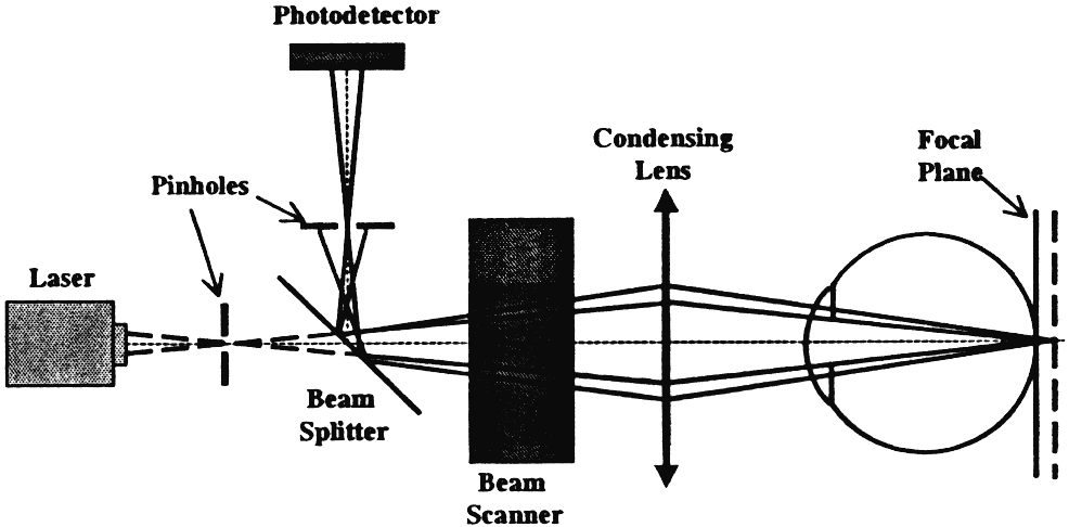
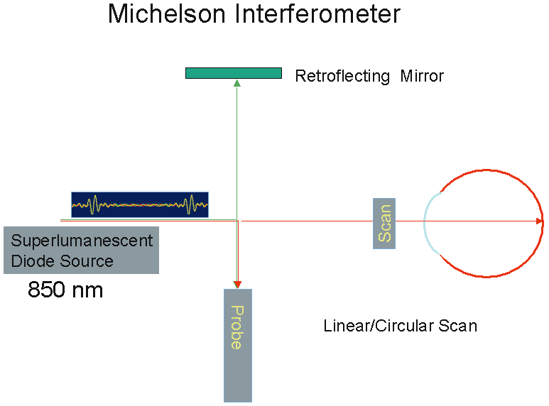
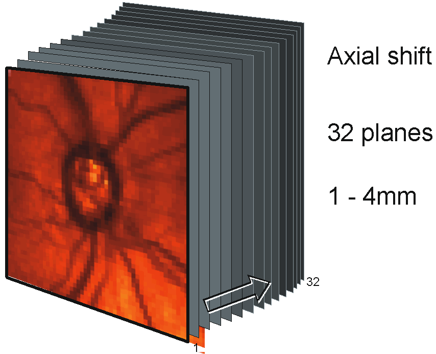
A series of two-dimensional confocal optical section images can be recorded sequentially by changing the location of the focal plane along the optical axis, progressing from anterior to the ONH, through the ONH and ending posterior to the lamina cribrosa. A tomographic series typically consists of 32 sequentially scanned optical section images, allowing the object to be resolved spatially in three dimensions. A mean topography image is typically produced from averaging three sets of three-dimensional images. With a current commercially available version, the Heidelberg Retina Tomograph (HRT) II (Heidelberg Engineering, Heidelberg, Germany), the field of view is fixed at 15 × 15 degrees, and digitization is performed in frames of 384 × 384 pixels with a spatial resolution of 10 μm per pixel. Image acquisition takes approximately 1 second. The scan depth, set by the operator, may range from 1 to 4 mm. The software stacks the series of 32 images so that corresponding points on the retina are aligned horizontally and vertically to compensate for eye movement during image acquisition (Fig. 2).

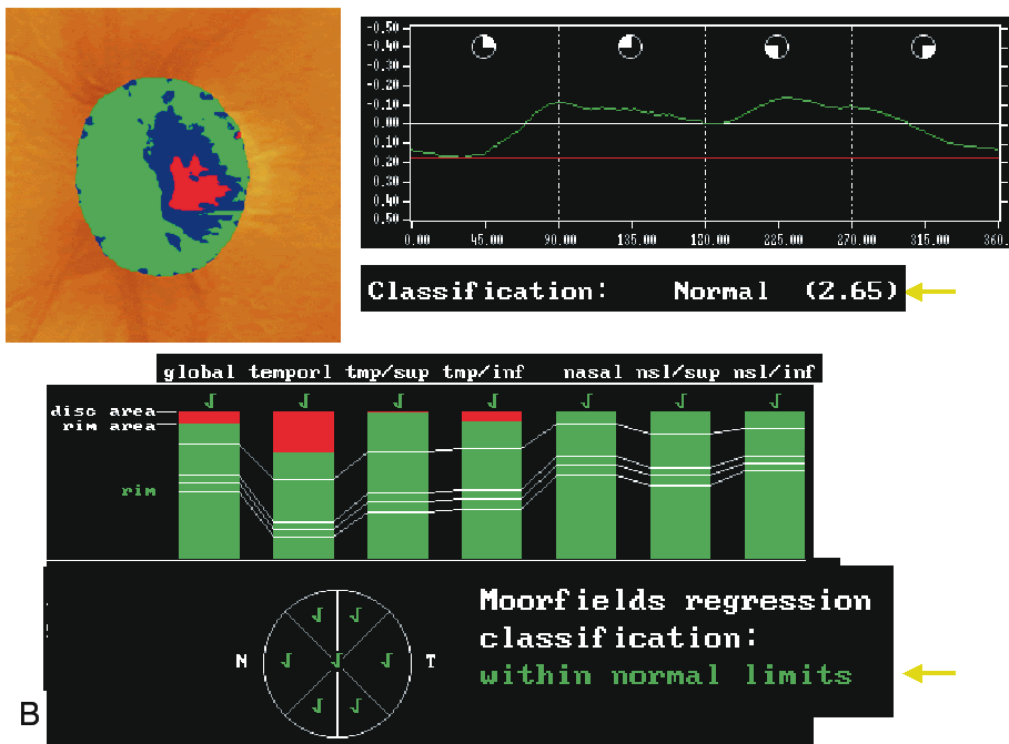
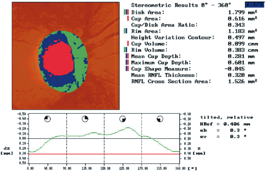
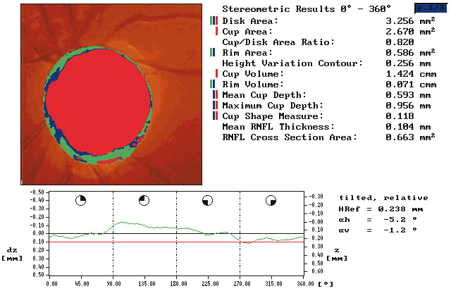
To evaluate the topographic information a contour line defining the disc margin is drawn by the examiner around the inner margin of the peripapillary scleral ring. The HRT software then establishes a reference plane 50 μm posterior to the retinal surface at the papillomacular bundle. The reference plane is established at this location because the fibers in the papillomacular bundle are thought to be least affected as glaucoma progresses, thereby providing a stable reference plane. As displayed in Figure 3, all structures below the reference plane are considered to belong to the optic cup (red) and all structures above the reference plane and within the contour line are considered to belong to neural rim (blue).

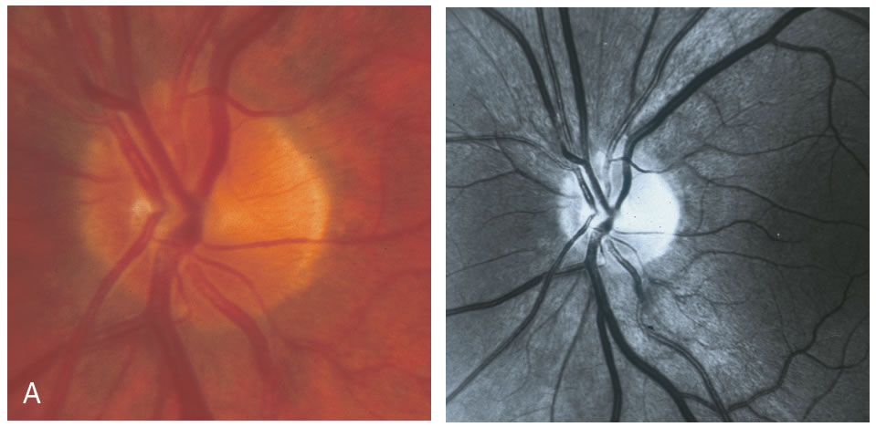
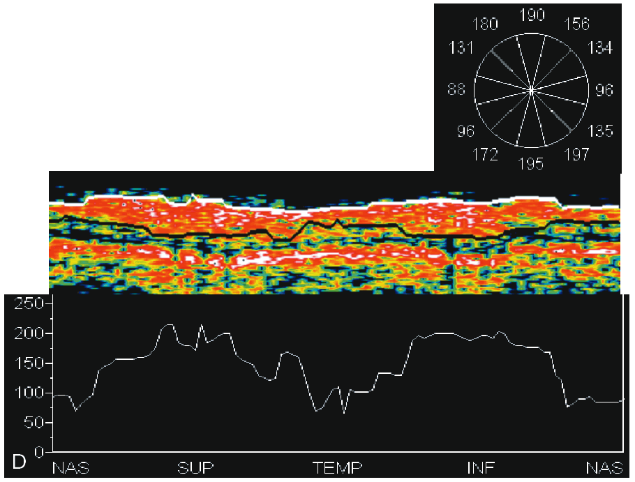
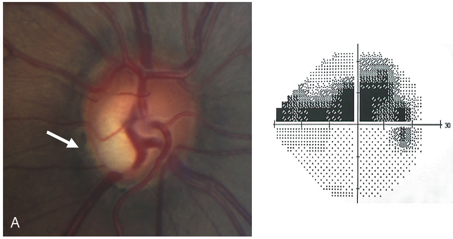
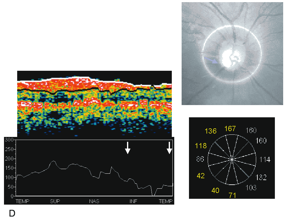
Stereometric parameters of optic nerve head topography are generated relative to the reference plane and include rim area, rim volume, cup area, cup volume, cup-to-disc ratio, mean RNFL thickness, and RNFL cross-sectional area. Parameters independent of the reference plane include mean and maximum cup depth, height variation contour, and cup shape measure (the statistical third moment of the distribution of all cup depth measurements). A characteristic sign in normal discs is the configuration of the contour line height display that demonstrates a double hump pattern corresponding to the thicker distribution of nerve fibers along the superior and inferior poles of the ONH (Fig. 4). Glaucomatous structural damage is characterized by a reduction of parameters that describe rim structures (area, volume) and indicate tissue loss (cup shape measure, cup volume, cup-to-disc ratio, cup steepness). As shown in Figure 5, glaucomatous alterations are typically associated with an asymmetrical or diffuse flattening of the contour line, or localized depressions corresponding to disc notches.

REPRODUCIBILITY

The reproducibility of a measurement is critical to determine the validity of a single measurement or to detect change in repeated measurements over time. With regard to optic nerve imaging, reproducibility is defined as the ability to obtain the same values in the absence of structural change. The magnitude of change that is detectable by the instrument is related to its reproducibility; the better the reproducibility the smaller the change that can be detected. Test-retest variability must, therefore, be small to detect small but real changes of the ONH to determine interval progression of glaucomatous damage. Various investigators have reported high levels of reproducibility with CSLO.^19–24 The reproducibility of height measurements has been shown to be between 10 and 20 μm and the coefficients of variation of the stereometric parameters been reported to be approximately 5%. Mean standard deviation of test-retest variability was found to be significantly greater for glaucoma patients versus normal controls.²⁵ Test-retest variability was also influenced by age, and was greater in older patients. Because glaucomatous discs tend to have a greater degree of sloping and excavation of the neural rim, and because the computer algorithm used to align the images has a higher error in areas of steep topographic slope, it is not surprising that glaucoma patients were found to have a higher degree of test-retest variability. The age effect was largely attributed to media opacities. No significant differences were found between short-term and long-term variability estimates, indicating that measurements are not influenced by the time interval between measurements.²⁶

ACCURACY

Histologic validation of measurements obtained with CSLO has been reported. Good correlation was found between in vivo optic disc topographic measures and histomorphometric measurements of optic nerve fiber number in primate eyes with laser-induced glaucoma.²⁷ Plastic models have also been developed which have shown high levels of accuracy with CSLO.²⁸ However, extrapolation of these results to a living human eye is difficult because of the different and complex optical properties of living human tissue.

Clinical correlation with CSLO measurements has concentrated on associations between topographic measures with visual function. A significant association between RNFL cross-sectional area and regional and hemifield measures of visual field loss has been reported.²⁹ Peripapillary height,³⁰ rim area and cup shape measure^31,32 have also been demonstrated to be highly correlated with global indices of visual function. Cup shape measure summarizes the structure of the cup and takes into account its depth variation and steepness of the cup walls, independent of both disc size and a retinal reference plane. This parameter is a good indicator of the severity of disc damage and appears to have parameter the strongest relationship with visual field loss.

SENSITIVITY AND SPECIFICITY

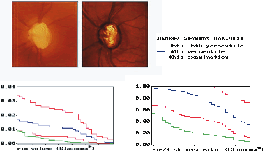
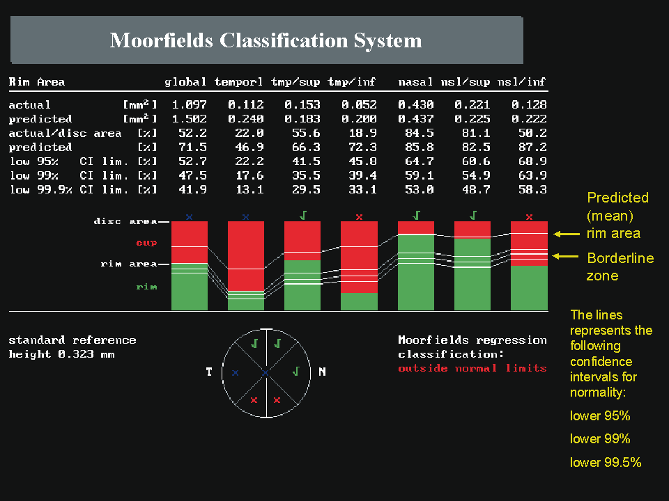
Because of the large interindividual variability of normal optic nerve head topography, there is no technique, qualitative or quantitative, that will provide perfect discrimination between normal and glaucomatous eyes. It is therefore not surprising that there is considerable overlap in individual optic disc parameter measurements between healthy eyes and eyes with early to moderate glaucoma. Currently, the HRT uses software with various statistical analyses to improve the discriminating ability between normal and glaucomatous eyes. These techniques include multivariate discriminant analysis, ranked segment distribution curves (Fig. 6), and regression analysis using a normative database (Fig. 7).

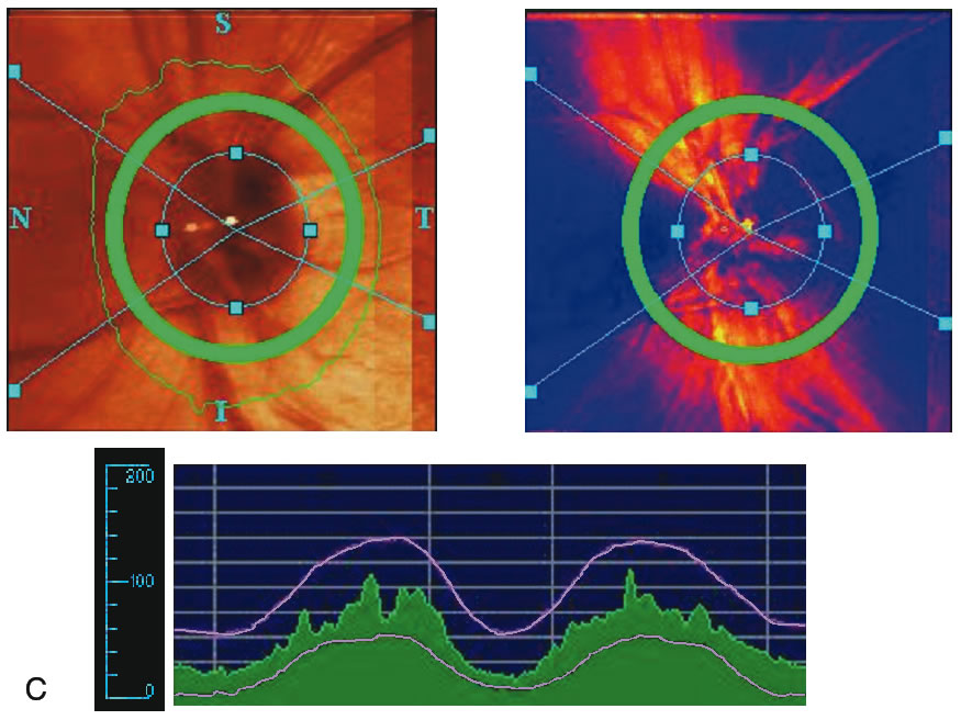
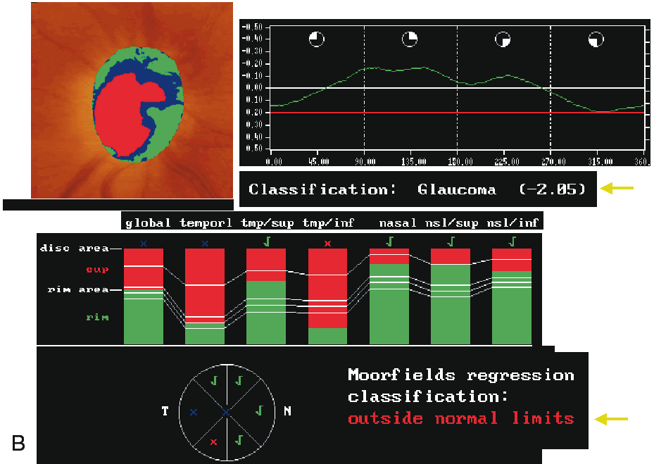
Multivariate analysis studies of the HRT parameters take into account combinations of parameters. It has been found by several investigators that cup shape measure, rim volume, and retinal height variation contour are the most important parameters to differentiate between normal and glaucomatous optic discs.^33-35 A linear combination of these parameters has been used to compute the Mikelberg discriminant function for classification of optic discs as normal or glaucomatous. With ranked segment distribution (RSD) curves, the optic nerve head is divided into 36 segments of 10 degrees, the stereometric parameters of which are then plotted in descending order. Each individual ranked segment analysis can then be compared to the normal range. An eye with glaucomatous damage is shown in Figure 6. The RSD curves are far outside the fifth percentile for normal eyes. This eye can therefore been classified as being glaucomatous with a probability of more than 95%.

Regression analysis was used to generate the Moorfield's regression classification score, which is based on the relationship between the neuroretinal rim area and the optic disc area. This classification system, as depicted in Figure 7, determines whether a disc is within or outside the normal reference limits derived from a normative database. Approximately 67% of eyes with early glaucoma are classified as outside normal limits and a further 20% are borderline.³⁶ Abnormalities other than glaucoma, such as tilted discs, may cause measurements to fall outside the normal range. The sensitivity and specificity of the HRT to discriminate between healthy and glaucomatous eyes has been investigated and varies widely, ranging from 62% to 84% and 80% to 96%, respectively (Table 1).^33,35–38 This wide variability in discriminating ability may be explained in part by different sample sizes, definitions of glaucoma, and varying degrees of glaucomatous optic nerve damage. It should be emphasized that the characteristics of the study population markedly influence the discriminating ability of any technique involved in differentiating glaucomatous from healthy eyes. For any technique, an instrument will appear to be more sensitive if it is used to separate healthy eyes from those with advanced glaucoma compared to those with only mild glaucoma.

Table 1. Confocal Scanning Laser Ophthalmoscopy: Previously Published Results of Sensitivity and Specificity

ABILITY TO DETECT CHANGE OVER TIME

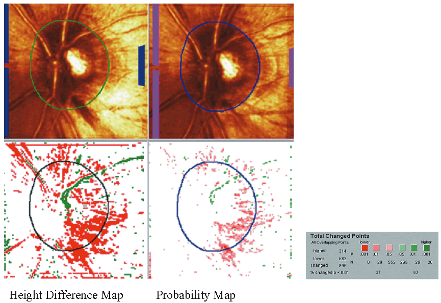
Quantitative methods that facilitate longitudinal analysis of topographic information are under active development. Longitudinal studies are underway to identify the best summary measurements to detect change and to determine whether CSLO can improve our ability to detect progression of glaucoma. Because progression of glaucoma is slow, years of follow-up are needed to answer this question. Follow-up studies in monkeys³⁹ and in patients after surgery^40,41 or medical reduction of intraocular pressure⁴² can be used as surrogates to more rapidly determine which analysis strategies are best to identify clinically relevant progression of glaucoma. Currently, there are several automated analysis strategies on the HRT to detect change in optic disc topography over time. These include topographic difference images, probablility map analysis and statistical changes in stereometric parameters.

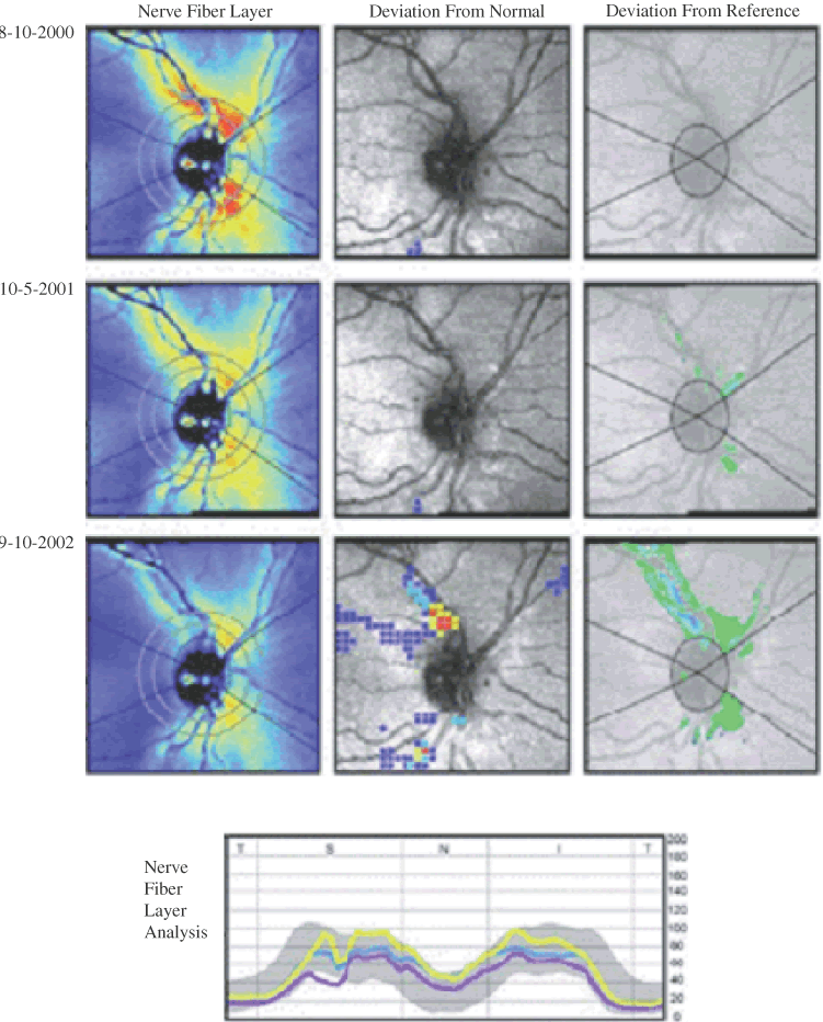
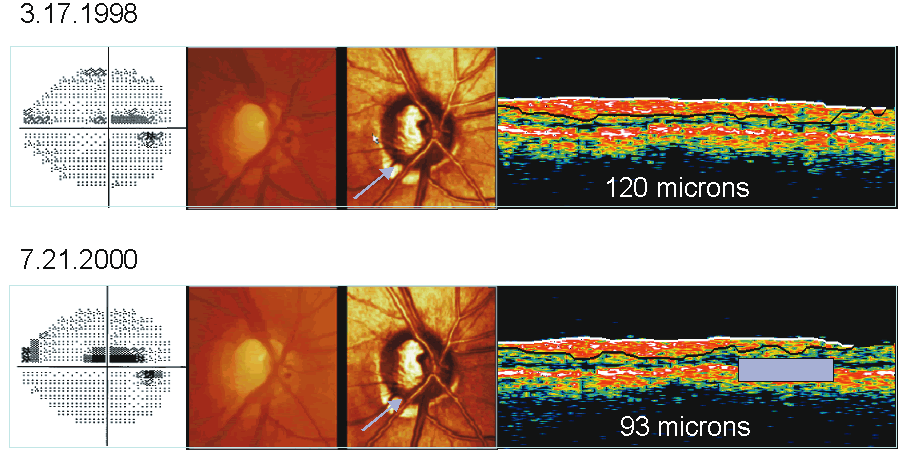
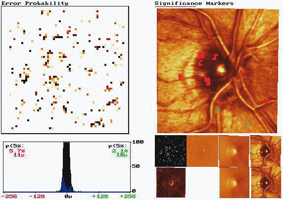
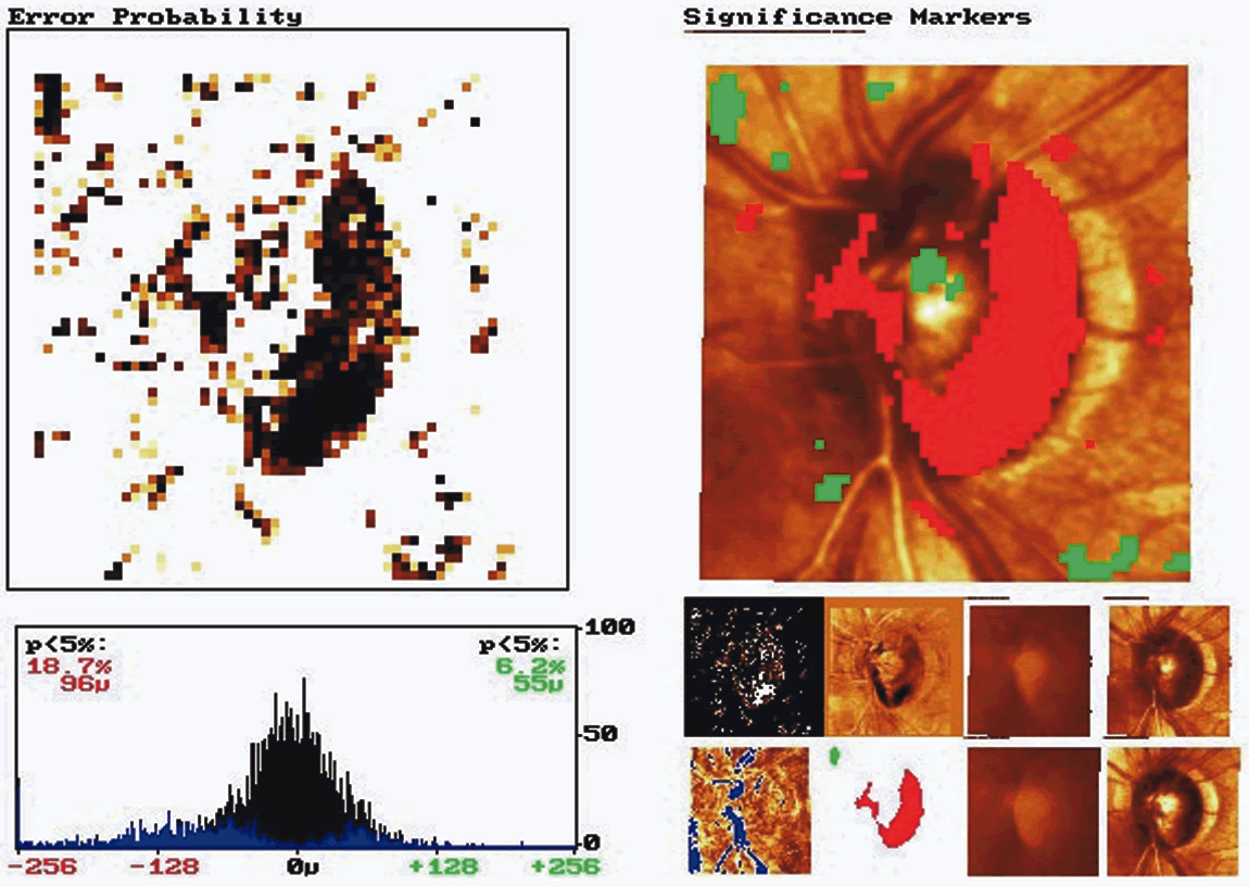
Topographic difference images are determined from the mean topographic images of at least two examinations after automatic correction for shift, rotation, and tilt between the images. Based on multiple image acquisitions during each visit, the software also determines the reproducibility for each individual examination at each location in the image by calculating the standard deviation of the height measurements. This allows the significance of a detected local height change to be determined and appropriate confidence intervals developed. Figure 8 shows the baseline and follow-up examination of a glaucomatous eye. The red areas on the height difference map are depressed more than 50 μm on the follow-up examination. The probability map, on the right, displays the significance of the detected change. The sensitivity for detecting change is influenced by the reproducibility of the height measurements. Therefore, in areas of greater variability, such as along the slope of the cup and over the blood vessels, the confidence limits of the measurement will be larger, and thus requires a greater change before it can be detected reliably.

Probability map analysis is based on the evaluation of arrays of condensed superpixels from individual topographic images from which location-specific confidence intervals have been determined. The analysis includes a color-coded image of change in condensed pixels over time that can be viewed with the probability map to determine which areas of change reach statistical significance. In the example in Figure 9, the baseline and follow-up examination of a normal eye are shown. This probability map is rather clean, with approximately 5% of the superpixels randomly spread over the entire image exhibiting significant change, reflecting a relatively small amount of noise inherent to the image. Figure 10 shows the probability map analysis of a glaucoma patient with 5 years between baseline and follow-up examinations. The red markers on the right in Figure 10 indicate diffuse glaucomatous progression of the neuroretinal rim. The advantage of topographic difference images and probability map analyses include their provision of location-specific change information. In addition, there is no need to outline the disc margin or to determine a reference plane.

Global and regional changes in stereometric optic disc parameters can be monitored over time. Analysis strategies that normalize parameters for graphical presentation with values of 0 for normal and 1 for glaucoma have recently been introduced, with most eyes assigned as intermediate value depending on whether they appear more normal or more glaucomatous.

ADVANTAGES

CSLO provides objective, reproducible, quantitative assessment of the ONH and RNFL. Real-time three-dimensional topographic maps of the ONH can be obtained in approximately 1 second. Images can be obtained even with moderate cataract and do not require pupillary dilation. No mechanical storage is necessary and multiple topographic summary parameters are obtainable with automated techniques.

DISADVANTAGES

The high cost has limited the generalized use of this technology in clinical practice. In addition, the considerable variation in optic disc topography among normal eyes necessitates a large age- and race-specific normative database that has yet to established. Further studies are needed to determine the most sensitive and specific summary measurements for diagnosis and management of glaucoma. Technological limitations include the use of a standard reference plane and the need for correct placement of the disc margin by the operator, both of which can influence many of the topographic indices generated. Assessment of optic disc topography is only one aspect of the clinical evaluation for glaucoma. Other features of glaucoma including RNFL damage, peripapillary atrophy, and disc hemorrhages can be missed by sole reliance on this technique for monitoring of glaucoma.

A 780-nm diode confocal scanning laser with an integrated polarimeter is focused on the retina. The backscattered light that doubly passes through the RNFL shows retardation that is linearly related to the RNFL and is measured by a polarization detection unit. The total data acquisition takes 0.7 seconds. Three images of each eye are obtained. Each image measures 15 × 15 degrees and contains 65,536 (256 × 256) pixels. These are displayed in a color-coded map. Areas of high retardation are displayed in yellow and white and areas of low retardation displayed in blue. A reflectance image of the scanned image is also produced. The operator outlines the optic disc margin and retardation values are automatically generated along a 10 pixel-wide ellipse, concentric with and 1.75 times larger than the disc diameter. The thickness values along the perimeter of the ellipse are then plotted as a cross-sectional graph. Figure 12 is an example of a healthy eye, demonstrating the typical eye double hump curve, representing a cross section of the two arcuate bundles, with the nasal, usually thinner, area in the center and the temporal area on the sides. Figure 13 is an example of a glaucomatous eye with thinning of the superotemporal neuroretinal rim with a corresponding inferonasal visual field defect. Retardation is markedly attenuated and the double hump curve is significantly depressed in the superotemporal quadrants.

In order to quantify retardation arising from only the RNFL, the corneal birefringence arising from the parallel arrangement of collagen fibers within the stroma must be accounted for.⁴³ An earlier version of the GDx Nerve Fiber Analyzer (Laser Diagnostic Tecnologies, San Diego, CA) used a corneal compensator with a fixed axis (15 degrees nasally downward) and a fixed magnitude of retardation (60 nm), so that the corneal component of retardation was eliminated only if the eye being imaged matched the population mode. However, a large variability of corneal birefringence exists in the population and if either the orientation or magnitude of retardation of the measured cornea lies outside the normal range, retardation resulting from the interaction of the cornea and the compensator will cause inaccurate estimations of RNFL thickness.⁴⁴ The GDx has recently been modified with a variable corneal compensator designed to provide individual corneal compensation. With two optical retarders, the variable corneal compensator neutralizes the residual corneal birefringence in each eye, calculated from the macular retardation pattern of that individual. The top image in Figure 14 shows an alteration in the normal retardation pattern of the macula as a result of uncompensated corneal birefringence. A supranormal retardation pattern is seen at the superior and inferior poles of the optic disc. The bottom image, with appropriate corneal compensation, depicts the normal macular retardation pattern caused by the radially arranged Henle fibers. A normal retardation pattern is seen at the optic disc. Early studies of the instrument with the variable corneal compensator have demonstrated that intersubject variability of measured RNFL thickness of normal eyes is reduced, the facility to discriminate between normal and glaucomatous eyes is improved, and the correlation of RNFL thickness values with visual function is greater.^45-49

A computer algorithm automatically generates retardation measurements throughout the peripapillary region and along the measurement ellipse. Average quadratic measurements, measurement ratios, symmetry measurements between superior and inferior quadrants, and modulation parameters are calculated. “The Number,” the result of an experimental neural network that is thought to reflect the probability of glaucoma on a scale of 0 to 100, is also generated.

REPRODUCIBILITY

High levels of reproducibility have been reported with SLP.^50,51 The within-pixel reproducibility of the third generation NFA, the GDx, has been reported to have a mean SD of only 5 μm.⁵² Of significance, the reproducibility of measurements was found to vary considerably across parameters. Reproducibility was not found to be consistently better or worse in normal or glaucomatous eyes. Intraoperator and interoperator reproducibility have also been assessed.⁵³ Intraoperator reproducibility of RNFL measurements was found to be good with all coefficients of variation being less than 10%. It was shown that interoperator error in image analysis could be reduced by using a single ellipse for the baseline and all subsequent scans even if subsequent scans were acquired by different operators.

ACCURACY

Histologic validation of retardation measurements obtained with SLP has been reported in two studies. RNFL thickness measurements were performed on two enucleated monkey eyes with the cornea and lens removed and a good correlation was found between RNFL thickness and retardation.⁵⁴ In the second study, with intact primate eyes, an inconsistent correlation was found between retardation and RNFL thickness with variation in the relationship between the two around the circumference of the optic disc.⁵⁵ In human postmortem eyes with the cornea and lens removed, the pattern of peripapillary retardation is consistent with known properties of the RNFL, with the slow axes of the birefringent structures in the peripapillary retina arranged radially around the optic disc.⁵⁶ In addition, an age-related decline in retardation has been reported,^50,57 that may result from the age-related loss of axons that has been demonstrated histologically.⁵⁸

Clinical correlation with SLP measurements has concentrated on associations of optic nerve structure with visual function. Early reports comparing visual field and NFA images found a moderate correlation.²⁹ More recently, SLP results correlated well with short wavelength perimetry and identified RNFL defects in eyes that did not show a defect on standard achromatic perimetry. A positive correlation between the visual field mean sensitivity and RNFL thickness determined by SLP was found, suggesting a critical RNFL thickness threshold, below which a precipitous decrease in visual field sensitivity occurs.⁵⁹

SENSITIVITY AND SPECIFICITY

Several investigators have provided estimates of sensitivity and specificity for detecting glaucoma with SLP (Table 2).^57,60–62 These studies have yielded a wide range of sensitivity and specificity. It is difficult to directly compare these reports because a number of different factors may have contributed to the variation in performance, such as the version of the instrument, analysis technique, sample size, degree, and type of glaucoma damage, as well as racial differences among study populations. In addition, reported sensitivities and specificities are usually obtained on only one population sample and not tested on another. Testing on other cohorts of subjects would allow for independent validation of estimates of sensitivity and specificity.

Table 2. Scanning Laser polarimetry: Previously Published Results of Sensitivity and Specificity

Because of the great variability in normal RNFL thickness, it is not surprising that when individual GDx parameters are used, SLP does not sufficiently discriminate normal from glaucomatous eyes.^60,62 Combining parameters and using various statistical analyses provides an increased specificity and increased diagnostic capacity. Constructed SLP parameters (modulation scores, ratio parameters) have been reported to have greater discriminating power than the retardation parameters which provide summary measures of RNFL thickness (average thickness and integral measurements).⁶³ Constructed retardation parameters have also been shown to have a better correlation with visual field mean defect.⁵³ This is explained by recent evidence suggesting that interindividual variability in corneal birefringence has falsely broadened the normative database of RNFL thickness assessments, and reduced the sensitivity and specificity of this technology. Correction for corneal polarization axis has been shown to significantly increase the correlation between RNFL structural damage and visual function, and significantly improve the discriminating power of SLP for detection of mild to moderate glaucoma.^45–49

The automated parameter, The Number, has been shown to perform better than many of the other individual parameters.⁶⁰ It is derived from a neural network of a large normative data set. This parameter provides an indicator of whether an eye is normal or glaucomatous by providing a rating on a scale of 0 to 100. According to the manufacturer, a number between 0 and 30 is normal, between 31 and 69 is suspicious, and 70 or greater is very suggestive of glaucoma. While The Number may be suitable for detecting diffuse RNFL abnormalities, it often fails to flag localized RNFL defects.⁶⁴ In a true screening situation, it is of concern that patients with a glaucomatous visual field defect from localized RNFL loss could be undetected with this approach.

ABILITY TO DETECT CHANGE OVER TIME

The RNFL measures can be compared over time by importing the operator-defined ellipse from the baseline image to all follow-up images and exporting summary parameter data for analysis. As shown in Figure 15, a serial printout is available that includes color-coded deviation from reference information for baseline and all follow-up examinations. After automatic image alignment, deviations from reference values are calculated by comparing pixel by pixel retardation measures over time between the baseline and follow-up images. Statistically significant values are calculated as thickness changes over time between the baseline and follow-up mean images compared with the overall standard deviation of the three individual images that comprise the mean image at baseline. The areas of statistically significant change are displayed. In order to differentiate change from measurement variability, change at a given location should be defined as repeatable and should require the involvement of several contiguous pixels.

Detection of change in the RNFL has been reported in eyes with nonglaucomatous optic neuropathy.^65,66 Progressive RNFL loss detected by SLP over a 90-day period was reported in a patient with traumatic optic neuropathy.⁶⁵ A second case over a 5-week period was described in a patient with acute nonarteritic anterior ischemic optic neuropathy with a corresponding dense altitudinal visual field depression.⁶⁶

ADVANTAGES

SLP provides a method of obtaining objective, quantitative, reproducible RNFL thickness measurements. The rapidity of image acquisition and the absence of a need for pupil dilation offer a distinct advantage over conventional photography. Multiple RNFL measurement parameters are available with automated software and the existence of a normative database allows comparison to nonglaucomatous eyes. Unlike CSLO, no correction for ocular magnification is required and a reference plane is not needed.

DISADVANTAGES

The considerable measurement variation between normal and glaucomatous eyes limits the usefulness of this technology as a single test to diagnose glaucoma. Ideal measurement parameters for glaucoma diagnosis and management remain to be established. The introduction of the variable corneal compensator has alleviated some of the concerns regarding the significant overlap of parameters among normal and glaucomatous eyes. However, the stability of compensation over time, as well as the influence of macular disease and refractive surgery on compensation, has not yet been determined. Currently, change analysis software lacks statistical units of change probability, making it difficult to differentiate true structural change from test-retest variability when performing serial analysis of absolute RNFL thickness values. Prospective studies are necessary to validate change analysis strategies.

An operator-determined circular or linear path is scanned across the retina to generate a series of 100 axial reflectance profiles. From these, a real-time two-dimensional tomographic image is constructed. Digital processing of the A-scans aligns them to correct for eye motion and pulsation by cross-correlating peaks between adjacent axial scans. A filter is applied to remove extreme values of reflectivity in the image. The layers of reflecting surfaces in the retina are given false colors to produce a map which is axially expanded. Tissues with high reflectivity are shown in white or red and those with low reflectivity are in blue or black. The axial resolution of OCT is of the order of 10 μm. The depth values of the scan are independent of the optical dimensions of the eye and no reference plane is required.

The pupil should be pharmacologically dilated during image acquisition to optimize optical alignment and avoid aberration caused by the pupillary edge. There is an internal and an external fixation target. The imaging lens is positioned 1 cm from eye to be examined and adjusted until the retina is in focus. An infrared-sensitive charge-coupled device (CCD) video camera displays the position of the scanning beam on retina. The first reflection measurement is the vitreoretinal interface that is demarcated by the contrast between the nonreflective vitreous and the high backscattering of the retinal surface. The highly reflective layer delineates the posterior boundary of the retina and corresponds to the retinal pigment epithelium. The inner margin of the retina shows another bright area of backscattering, a thin layer, that corresponds to the RNFL. Figure 17 is an example of a healthy eye in which the anterior and posterior highly reflecting layers can be seen (shown in red), representing the RNFL and retinal pigment epithelium, respectively. The inferotemporal and superotemporal nerve fiber bundles are evident as localized thickenings in both the RNFL and the retina. Figure 18 is an example of a glaucomatous eye with a broad focal defect in the superotemporal quadrant with thinning of the RNFL to less than 50 μm.

RNFL thickness may be assessed from a circular or linear tomogram in the peripapillary region. A circular scan around the ONH allows the variations in RNFL thickness in different regions around the disc to be assessed and compared, whereas a linear tomogram through the optic disc provides cross-sectional information for assessing disc and cup parameters (Fig. 19). Computer-generated profiles of the RNFL and retinal boundaries can automatically identify the reflective boundaries at the vitreoretinal interface, the retinal pigment epithelium and the RNFL. RNFL or retinal thickness can be computed automatically from these boundaries and can be displayed as averaged over quadrants or clock hours. These quantitative measurements can then be compared with standard normal values or values obtained from previous examinations.

REPRODUCIBILITY

High levels of reproducibility have been reported with OCT. Standard deviations of repeated measurements are between 10 to 20 μm for overall RNFL thickness and 5 to 9 μm for retinal thickness. A circle diameter of 3.4 mm was found to be superior to other scan diameters and internal fixation was significantly less variable than external fixation.⁶⁷ The coefficient of variation for mean RNFL thickness has been reported to about 12% in glaucomatous eyes and somewhat smaller in normal eyes (7%).^{68, 69}

It has been shown that increased sampling density improves the reproducibility of OCT measurement in glaucomatous eyes.⁷⁰ Different sampling densities have been studied: quadrantic scans with 100 sampling points per quadrant and circular scans with 25 points per quadrant. No differences in RNFL thickness measurements and coefficient of variation between the two techniques were found in normal eyes. In glaucomatous eyes, however, the coefficient of variation in the scans with 25 sampling points per quadrant (25.9%) was significantly higher than that in the scans with 100 sampling points per quadrant scans (11.9%).

ACCURACY

Histologic validation of retinal thickness measurements obtained with OCT has been reported. The ability of OCT to detect progressive RNFL loss in an experimental model of primate glaucoma eyes has been evaluated.⁶⁷ OCT demonstrated a linear reduction in RNFL thickness over time in eyes with increased IOP compared to control eyes in which there were no detectable changes. Correlation between OCT measurements and histopathologic examination revealed agreement for RNFL thicknesses within 10 μm.

Structural measurements with OCT correspond with known properties of the RNFL. Thickness measurements decrease with increasing distance from the ONH⁶⁷ and with increasing age.⁷¹ RNFL thickness measurements in glaucomatous eyes are significantly less compared to normal eyes, and there is good correlation between thickness measurements and visual function.⁷¹ A number of reports have demonstrated good correlation between retinal thickness measurements and conventional qualitative measurements of retinal pathology in such conditions as macular edema,⁷² macular holes,⁷³ and epiretinal membranes.⁷⁴

SENSITIVITY AND SPECIFICITY

Several investigators have provided estimates of sensitivity and specificity for detecting glaucoma with OCT, yielding fairly consistent results (Table 3).^63,75,76 The inferior quadrant thickness parameters have been found to best discriminate between normal and glaucomatous eyes. Combinations of parameters have also been evaluated with more controversial results. In one such study, the best OCT analysis was derived from discriminant analysis of RNFL thickness in 30-degree sectors.⁷⁶ Another investigator found that no combination of parameters resulted in greater discriminating ability than the single best individual parameter.⁷⁵

Table 3. Ocular Coherence Tomography: Previously Published Results of Sensitivity and Specificity

RNFL thickness measured with OCT has been assessed and compared in normal, ocular hypertensive and glaucomatous eyes. Several investigators have shown that OCT is capable of differentiating glaucomatous from non-glaucomatous eyes, and that OCT RNFL thickness measurements correlate with SLP retardation measurements and CSLO topographic measurements.^{77, 78} In glaucomatous eyes, RNFL was found to be significantly thinner than both ocular hypertensive and normal eyes in all four quadrants. The RNFL has also been found to be significantly thinner in ocular hypertensive than in normal eyes in the inferior and nasal quadrants. It is possible that thinner RNFL in the inferior quadrant of OHT eyes detected by OCT is an early form of glaucoma that precedes detectable optic nerve or visual field defects.⁷⁹

ABILITY TO DETECT CHANGE

Change analysis software for the OCT has only recently been introduced and, thus far, there are no reports describing longitudinal change in patients with disease progression. The new algorithm generates a serial analysis of RNFL thickness measurements between two OCT images. However, statistical units of change probability are not provided and it is difficult to differentiate true physiologic change from test-retest variability. Figure 20 shows a baseline and follow-up image of an uncontrolled glaucomatous eye after a 16-month interval. Thinning of the RNFL in the inferotemporal quadrant is seen with worsening of the corresponding superior arcuate visual field defect.

ADVANTAGES

OCT provides objective, quantitative, reproducible measurements of the retina and RNFL thickness. In contrast with other imaging techniques, direct measurements of the RNFL are calculated from cross sectional retinal images. Measurements are not affected by refractive status, axial length of the eye or the presence of moderate nuclear sclerotic cataracts. An anterior segment compensator is unnecessary and structural information is independent of a reference plane.

DISADVANTAGES

As with other ocular imaging technology, high cost precludes generalized use of the OCT in the clinical arena. The presence of posterior subcapsular and cortical cataracts impairs performance⁶⁷ and pupillary dilation is required to obtain acceptable peripapillary measurement scans. OCT images contain significantly fewer pixels than both SLP and CSLO. Recent evidence suggests that increasing the sampling density of OCT scans from 25 points per quadrant to 100 points per quadrant provides a less variable representation of RNFL thickness.⁷⁰ Currently change analysis software lacks statistical units of change probability, making it difficult to differentiate biological change from measurement variability. In addition, the absence of a large age- and race-specific normative database is a limitation of this technology.

Comparative studies that examine the diagnostic performance of various instruments in a single population are advantageous in that they eliminate population-characteristic–based variables, allowing a direct comparison of results obtained with the different instruments. It should be recognized, however, that the different diagnostic technologies are at different stages of development with the more established technologies benefiting from more robust normative databases and more sophisticated analysis strategies.

Figures 21 and 22 are examples of both a normal and glaucomatous eye with images taken from all three instruments. In Figure 22, marked thinning of the inferior neuroretinal rim is seen in the glaucomatous eye with a notch at the 7 o'clock position. There is a corresponding superior arcuate defect on visual field testing. The optic disc is classified as outside normal limits by HRT with Moorfield's classification system. Attenuation of retardation and a flattening of the double hump curve in the inferotemporal region is noted on SLP. The OCT shows a reduction of the nerve fiber layer in this region to 40 μm.

Fig. 21. Comparison of imaging techniques: healthy eye. A. A healthy appearing neuroretinal rim is seen. B. The optic disc is classified as within normal limits by Heidelberg Retina Tomograph (HRT; Heidelberg Engineering, Heidelberg, Germany) with Moorfield's classification system. C. A typical double hump curve is seen on scanning laser polarimetry (SLP). D. The anterior and posterior highly reflecting layers, representing the retinal nerve fiber layer (RNFL) and retinal pigment epithelium (RPE), can be seen on optical coherence tomography (OCT).

Fig. 22. Comparison of imaging techniques: glaucomatous eye. A. Marked thinning of the inferior neuroretinal rim is seen in this glaucomatous eye with a notch at the 7 o'clock position. There is a corresponding superior arcuate defect on visual field testing. B. The optic disc is classified as outside normal limits by Heidelberg Retina Tomograph (HRT; Heidelberg Engineering, Heidelberg, Germany) with Moorfield's classification system. C. Attenuation of retardation and a flattening of the double hump curve in the inferotemporal region are noted on scanning laser polarimetry (SLP). D. The optical coherence tomography (OCT) shows a reduction of the nerve fiber layer in this region to 40 μm.

At the present time, there is no consensus regarding the best method for the evaluation of glaucomatous structural damage. Moreover, the best summary measures for any given instrument have yet to be determined. The parameter or technique most useful in the detection of glaucomatous damage for one individual may differ from the next and may vary from those most useful for detection of glaucomatous damage at different stages. Available imaging technologies show considerable promise for the detection of glaucomatous progression over time. Analytic strategies for detection of change exist but have not yet been prospectively validated in large populations. Furthermore, new methods for detection of progression need to be compared to the current gold standard for both structural and psychophysical change. Statistical units of change probability are critical to differentiate true pathological change from test-retest variability. Constant improvements in available imaging instruments make it difficult to follow subjects longitudinally, as changes in software and hardware may alter baseline measurements.

In summary, each quantitative imaging technique of the optic nerve has its own advantages and disadvantages. Different instruments and various analysis strategies may be more effective in different situations. Each technique shows promise for the detection of glaucomatous progression given their high measurement reproducibility. It is not recommended that clinical decisions be based on the results of any single imaging test, as with visual field testing. Clinical correlation is essential and management must be tailored to each individual patient.

1. Hart WM Jr , Yablonski M, Kass MA, et al: Quantitative visual field and optic disc correlates early in glaucoma. Arch Ophthalmol 96:2209, 1978

2. Sommer A, Pollack I, Maumenee AE: Optic disc parameters and onset of glaucomatous field loss. I. Methods and progressive changes in disc morphology. Arch Ophthalmol 97:1444, 1979

3. Pederson JE, Anderson DR: The mode of progressive disc cupping in ocular hypertension and glaucoma. Arch Ophthalmol 98:490, 1980

4. Zeyen TG, Caprioli J: Progression of disc and field damage in early glaucoma. Arch Ophthalmol 111:62, 1993

5. Sommer A, Katz J, Quigley HA, et al: Clinically detectable nerve fiber atrophy precedes the onset of glaucomatous field loss. Arch Ophthalmol 109:77, 1991

6. Quigley HA, Katz J, Derick RJ, et al: An evaluation of optic disc and nerve fiber layer examinations in monitoring progression of early glaucoma damage. Ophthalmology 99:19, 1992

7. Airaksinen P, Tuulonen A, Alanko H: Rate and pattern of neuroretinal rim area decrease in ocular hypertension and glaucoma. Arch Ophthalmol 110:206, 1992

8. Lichter PR: Variability of expert observers in evaluating the optic disc. Trans Am Ophthalmol Soc 74:532, 1976

9. Varma R, Steinmann WC, Scott IU: Expert agreement in evaluating the optic disc for glaucoma. Ophthalmology 99:215, 1992

10. Tielsch JM, Katz J, Quigley HA, et al: Intraobserver and interobserver agreement in measurement of optic disc characteristics. Ophthalmology 95:350, 1988

11. Balazsi AG, Drance SM, Schulzer M, et al: Neuroretinal rim area in suspected glaucoma and early chronic open-angle glaucoma. Correlation with parameters of visual function. Arch Ophthalmol 102:1011, 1984

12. Garway-Heath DF, Hitchings RA: Quantitative evaluation of the optic nerve head in early glaucoma. Br J Ophthalmol 82:352, 1998

13. Airaksinen PJ, Drance SM: Neuroretinal rim area and retinal nerve fiber layer in glaucoma. Arch Ophthalmol 103:203, 1985

14. Varma R, Spaeth GL, Steinmann WC, et al: Agreement between clinicians and an image analyzer in estimating cup-to-disc ratios. Arch Ophthalmol 107:526, 1989

15. Dandona L: Reliability of optic nerve head topographic measurements with computerized image analysis. Am J Ophthalmol 108:414, 1989

16. Zeimer R, Asrani S, Zou S, et al: Quantitative detection of glaucomatous damage at the posterior pole by retinal thickness mapping. A pilot study. Ophthalmology 105:224, 1998

17. Brusini P: Quantitative mapping of the retinal thickness at the posterior pole in chronic open angle glaucoma. Acta Ophthalmol Scand Suppl 232:42, 2002

18. Zeimer R: A new method for rapid mapping of the retinal thickness at the posterior pole. Invest Ophthalmol 37:1994, 1996

19. Lusky M: Reproducibility of optic nerve head topography measurements in eyes with undilated pupils. J Glaucoma 2:104, 1993

20. Mikelberg F: Reproducibility of topographic parameters obtained with the Heidelberg Retina Tomograph. J Glaucoma 2:101, 1993

21. Dreher A: Reproducibility of topographic measurements of the normal and glaucomatous optic nerve head with the laser tomographic scanner. Am J Ophthalmol 111:221, 1991

22. Weinreb RN, Lusky M, Bartsch DU, et al: Effect of repetitive imaging on topographic measurements of the optic nerve head. Arch Ophthalmol 111:636, 1993

23. Brigatti L, Weitzman M, Caprioli J: Regional test-retest variability of confocal scanning laser tomography. Am J Ophthalmol 120:433, 1995

24. Cioffi G: Confocal laser scanning ophthalmoscope: Reproducibility of optic nerve head topographic measurements with confocal laser scanning ophthalmoscope. Ophthalmology 100:57, 1993

25. Chauhan BC, LeBlanc RP, McCormick TA, et al: Test-retest variability of topographic measurements with confocal scanning laser tomography in patients with glaucoma and control subjects. Am J Ophthalmol 118:9, 1994

26. Chauhan B: Influence of time separation on variability estimates of topographic measurements with confocal laser scanning tomography. J Glaucoma 4:189, 1995

27. Yucel YH, Gupta N, Kalichman MW, et al: Relationship of optic disc topography to optic nerve fiber number in glaucoma. Arch Ophthalmol 116:493, 1998

28. Janknecht P, Funk J: Optic nerve head analyser and Heidelberg retina tomograph: accuracy and reproducibility of topographic measurements in a model eye and in volunteers. Br J Ophthalmol 78:760, 1994

29. Weinreb RN, Shakiba S, Sample PA, et al: Association between quantitative nerve fiber layer measurement and visual field loss in glaucoma. Am J Ophthalmol 120:732, 1995

30. Tsai C: Correlation of peripapillary retinal height and visual field in glaucoma and normal subjects. J Glaucoma 4:110, 1995

31. Iester M, Mikelberg FS, Courtright P, et al: Correlation between the visual field indices and Heidelberg retina tomograph parameters. J Glaucoma 6:78, 1997

32. Uchida H, Tomita G, Onda E, et al: Relationship of nerve fiber layer defects and parafoveal visual field defects in glaucomatous eyes. Jpn J Ophthalmol 40:548, 1996

33. Bathija R, Zangwill L, Berry CC, et al: Detection of early glaucomatous structural damage with confocal scanning laser tomography. J Glaucoma 7:121, 1998

34. Vihanninjoki K, Teesalu P, Burk RO, et al: Search for an optimal combination of structural and functional parameters for the diagnosis of glaucoma. Multivariate analysis of confocal scanning laser tomograph, blue-on-yellow visual field and retinal nerve fiber layer data. Graefes Arch Clin Exp Ophthalmol 238:477, 2000

35. Iester M, Mikelberg FS, Swindale NV, et al: ROC analysis of Heidelberg Retina Tomograph optic disc shape measures in glaucoma. Can J Ophthalmol 32:382, 1997

36. Wollstein G, Garway-Heath DF, Fontana L, et al: Identifying early glaucomatous changes. Comparison between expert clinical assessment of optic disc photographs and confocal scanning ophthalmoscopy. Ophthalmology 107:2272, 2000

37. Iester M, Mikelberg FS, Drance SM: The effect of optic disc size on diagnostic precision with the Heidelberg retina tomograph. Ophthalmology 104:545, 1997

38. Caprioli J, Park HJ, Ugurlu S, et al: Slope of the peripapillary nerve fiber layer surface in glaucoma. Invest Ophthalmol Vis Sci 39:2321, 1998

39. Burgoyne CF, Quigley HA, Thompson HW, et al: Early changes in optic disc compliance and surface position in experimental glaucoma. Ophthalmology 102:1800, 1995

40. Lesk MR, Spaeth GL, Azuara-Blanco A, et al: Reversal of optic disc cupping after glaucoma surgery analyzed with a scanning laser tomograph. Ophthalmology 106:1013, 1999

41. Irak I, Zangwill L, Garden V, et al: Change in optic disk topography after trabeculectomy. Am J Ophthalmol 122:690, 1996

42. Bowd C, Weinreb RN, Lee B, et al: Optic disk topography after medical treatment to reduce intraocular pressure. Am J Ophthalmol 130:280, 2000

43. Knighton RW, Huang X, Zhou Q: Microtubule contribution to the reflectance of the retinal nerve fiber layer. Invest Ophthalmol Vis Sci 39:189, 1998

44. Greenfield DS, Knighton RW, Huang XR: Effect of corneal polarization axis on assessment of retinal nerve fiber layer thickness by scanning laser polarimetry. Am J Ophthalmol 129:715, 2000

45. Weinreb RN, Bowd C, Zangwill LM: Scanning laser polarimetry in monkey eyes using variable corneal polarization compensation. J Glaucoma 11:378, 2002

46. Garway-Heath DF, Greaney MJ, Caprioli J: Correction for the erroneous compensation of anterior segment birefringence with the scanning laser polarimeter for glaucoma diagnosis. Invest Ophthalmol Vis Sci 43:1465, 2002

47. Greenfield DS, Knighton RW, Feuer WJ, et al: Correction for corneal polarization axis improves the discriminating power of scanning laser polarimetry. Am J Ophthalmol 134:27, 2002

48. Weinreb RN, Bowd C, Greenfield DS, et al: Measurement of the magnitude and axis of corneal polarization with scanning laser polarimetry. Arch Ophthalmol 120:901, 2002

49. Zhou Q, Weinreb RN: Individualized compensation of anterior segment birefringence during scanning laser polarimetry. Invest Ophthalmol Vis Sci 43:2221, 2002

50. Weinreb RN, Shakiba S, Zangwill L: Scanning laser polarimetry to measure the nerve fiber layer of normal and glaucomatous eyes. Am J Ophthalmol 119:627, 1995

51. Zangwill L, Berry CA, Garden VS, et al: Reproducibility of retardation measurements with the nerve fiber analyzer II. J Glaucoma 6:384, 1997

52. Colen TP, Tjon-Fo-sang MJ, Mulder PG, et al: Reproducibility of measurements with the nerve fiber analyzer (NfA/GDx). J Glaucoma 9:363, 2000

53. Hoh ST, Ishikawa H, Greenfield DS, et al: Peripapillary nerve fiber layer thickness measurement reproducibility using scanning laser polarimetry. J Glaucoma 7:12, 1998

54. Weinreb RN, Dreher AW, Coleman A, et al: Histopathologic validation of Fourier-ellipsometry measurements of retinal nerve fiber layer thickness. Arch Ophthalmol 108:557, 1990

55. Morgan JE, Waldock A, Jeffery G, et al: Retinal nerve fibre layer polarimetry: Histological and clinical comparison. Br J Ophthalmol 82:684, 1998

56. Dreher A: Assessment of the retinal nerve fiber layer by scanning -laser polarimetry. SPIE 1877:266, 1993

57. Tjon-Fo-Sang MJ, de Vries J, Lemij HG: Measurement by nerve fiber analyzer of retinal nerve fiber layer thickness in normal subjects and patients with ocular hypertension. Am J Ophthalmol 122:220, 1996

58. Balazsi AG, Rootman J, Drance SM, et al: The effect of age on the nerve fiber population of the human optic nerve. Am J Ophthalmol 97:760, 1984

59. Kwon YH, Hong S, Honkanen RA, et al: Correlation of automated visual field parameters and peripapillary nerve fiber layer thickness as measured by scanning laser polarimetry. J Glaucoma 9:281, 2000

60. Trible JR, Schultz RO, Robinson JC, et al: Accuracy of scanning laser polarimetry in the diagnosis of glaucoma. Arch Ophthalmol 117:1298, 1999

61. Yamada N, Chen PP, Mills RP, et al: Glaucoma screening using the scanning laser polarimeter. J Glaucoma 9:254, 2000

62. Weinreb RN, Zangwill L, Berry CC, et al: Detection of glaucoma with scanning laser polarimetry. Arch Ophthalmol 116:1583, 1998

63. Bowd C, Zangwill LM, Berry CC, et al: Detecting early glaucoma by assessment of retinal nerve fiber layer thickness and visual function. Invest Ophthalmol Vis Sci 42:1993, 2001

64. Nicolela MT, Martinez-Bello C, Morrison CA, et al: Scanning laser polarimetry in a selected group of patients with glaucoma and normal controls. Am J Ophthalmol 132:845, 2001

65. Medeiros FA, Susanna R Jr : Retinal nerve fiber layer loss after traumatic optic neuropathy detected by scanning laser polarimetry. Arch Ophthalmol 119:920, 2001

66. Colen TP, van Everdingen JA, Lemij HG: Axonal loss in a patient with anterior ischemic optic neuropathy as measured with scanning laser polarimetry. Am J Ophthalmol 130:847, 2000

67. Schuman JS, Pedut-Kloizman T, Hertzmark E, et al: Reproducibility of nerve fiber layer thickness measurements using optical coherence tomography. Ophthalmology 103:1889, 1996

68. Baumann M, Gentile RC, Liebmann JM, et al: Reproducibility of retinal thickness measurements in normal eyes using optical coherence tomography. Ophthalmic Surg Lasers 29:280, 1998

69. Blumenthal EZ, Williams JM, Weinreb RN, et al: Reproducibility of nerve fiber layer thickness measurements by use of optical coherence tomography. Ophthalmology 107:2278, 2000

70. Gurses-Ozden R, Ishikawa H, Hoh ST, et al: Increasing sampling density improves optical coherence tomography measurement reproducibility. J Glaucoma 8:238, 1999

71. Schuman JS, Hee MR, Puliafito CA, et al: Quantification of nerve fiber layer thickness in normal and glaucomatous eyes using optical coherence tomography. Arch Ophthalmol 113:586, 1995

72. Hee MR, Puliafito CA, Wong C, et al: Quantitative assessment of macular edema with optical coherence tomography. Arch Ophthalmol 113:1019, 1995

73. Hee MR, Puliafito CA, Wong C, et al: Optical coherence tomography of macular holes. Ophthalmology 102:748, 1995

74. Wilkins J, Puliafito CA, Hee MR, et al: Characterization of epiretinal membranes using optical coherence tomography. Ophthalmology 103: 2142, 1996

75. Zangwill LM, Bowd C, Berry CC, et al: Discriminating between normal and glaucomatous eyes using the Heidelberg Retina Tomograph, GDx Nerve Fiber Analyzer, and Optical Coherence Tomograph. Arch Ophthalmol 119:985, 2001

76. Greaney MJ, Hoffman DC, Garway-Heath DF, et al: Comparison of optic nerve imaging methods to distinguish normal eyes from those with glaucoma. Invest Ophthalmol Vis Sci 43:140, 2002

77. Mistlberger A, Liebmann JM, Greenfield DS, et al: Heidelberg retina tomography and optical coherence tomography in normal, ocular-hypertensive, and glaucomatous eyes. Ophthalmology 106:2027, 1999

78. Hoh ST, Greenfield DS, Mistlberger A, et al: Optical coherence tomography and scanning laser polarimetry in normal, ocular hypertensive, and glaucomatous eyes. Am J Ophthalmol 129:129, 2000

79. Bowd C, Weinreb RN, Williams JM, et al: The retinal nerve fiber layer thickness in ocular hypertensive, normal, and glaucomatous eyes with optical coherence tomography. Arch Ophthalmol 118:22, 2000